Linear Regression and the Capital Asset Pricing Model (CAPM)

library(mosaic)   # Load additional packages here
library(tidyverse)  # Loads tidyquant, tidyverse, lubridate, xts, quantmod, TTR
library(ggformula)
library(GGally)
library(tidyquant)
library(ggfortify)
library(tinytex)

options(scipen=999)

# Some customization.  You can alter or delete as desired (if you know what you are doing).
knitr::opts_chunk$set(
  tidy=FALSE,     # display code as typed
  size="small")   # slightly smaller font for code
Introduction to the Capital Asset Pricing Model (CAPM)
A fundamental idea in finance is that investors need financial incentives to take on risk. Thus, the expected return R on a risky investment, e.g., a stock, should exceed the risk-free return Rf, or the excess return (R - Rf) should be positive. Typically, for risk-free rate we use short-term government bonds, like the US 3-month treasury bills https://finance.yahoo.com/quote/%5EIRX?p=^IRX
The Capital Asset Market Pricing Model (CAPM) states that the return on a particular risky asset is related to returns of the ‘market’ as follows:
\(Return(asset) = \alpha + \beta*Return(market)+error\)
The \(\alpha\) is the “excess return” of a stock. According to the CAPM, this “excess return” is the reward for taking on the “specific risk” of the stock. As this risk can be eliminated through holding a diversified portfolio, CAPM says the excess return should be close to zero.
The \(\beta\) is a measure of the “market risk” of a stock. It is an indication of how sensitive the stock is to movements in the market as a whole; for a 1% market movement, \(\beta=1\) implies the stock tends to move 1%, \(\beta<1\) means the stock tends to move by less than 1%, whereas \(\beta>1\) means the stock tends to move more than 1%, or it ‘exaggerates’ market movements.
We will run linear regressions to estimate the \(\alpha\) and \(\beta\) of a couple of stocks, as well as their specific risk. We will use the tidyquant package to download historical prices off the internet and will also see some R code that allows us to calculate a rolling beta. We will explore the relationship between returns (%) of the market (SPY, an ETF that tracks the S&P500) and for a number of stocks, namely Apple (ticker symbol: AAPL), JPMorgan (JPM), Disney (DIS), Domino’s Pizza (DPZ), and Abercrombie & Fitch Co. (ANF).
Loading the data
The tidyquant package comes with a number of functions, utilities that allow us to download financial data off the web, as well as ways of handling all this data.
We begin by loading the data set into the R workspace. We create a collection of stocks with their ticker symbols and then use the piping operator %>% to use tidyquant’s tq_get to donwload historical data from Jan 1, 2011 to Dec 31, 2017 using Yahoo finance and, again, to group data by their ticker symbol.
myStocks <- c("AAPL","JPM","DIS","DPZ","ANF","SPY" ) %>%
  tq_get(get  = "stock.prices",
         from = "2017-08-01",
         to   = "2020-09-30") %>%
  group_by(symbol)

str(myStocks) # examine the structure of the resulting data frame
## tibble [4,782 × 8] (S3: grouped_df/tbl_df/tbl/data.frame)
## $ symbol : chr [1:4782] "AAPL" "AAPL" "AAPL" "AAPL" ...
## $ date : Date[1:4782], format: "2017-08-01" "2017-08-02" ...
## $ open : num [1:4782] 37.3 39.8 39.3 39 39.3 ...
## $ high : num [1:4782] 37.6 39.9 39.3 39.3 39.7 ...
## $ low : num [1:4782] 37.1 39 38.8 38.9 39.2 ...
## $ close : num [1:4782] 37.5 39.3 38.9 39.1 39.7 ...
## $ volume : num [1:4782] 141474400 279747200 108389200 82239600 87481200 ...
## $ adjusted: num [1:4782] 35.9 37.6 37.2 37.4 38 ...
## - attr(*, "groups")= tibble [6 × 2] (S3: tbl_df/tbl/data.frame)
## ..$ symbol: chr [1:6] "AAPL" "ANF" "DIS" "DPZ" ...
## ..$ .rows : list<int> [1:6]
## .. ..$ : int [1:797] 1 2 3 4 5 6 7 8 9 10 ...
## .. ..$ : int [1:797] 3189 3190 3191 3192 3193 3194 3195 3196 3197 3198 ...
## .. ..$ : int [1:797] 1595 1596 1597 1598 1599 1600 1601 1602 1603 1604 ...
## .. ..$ : int [1:797] 2392 2393 2394 2395 2396 2397 2398 2399 2400 2401 ...
## .. ..$ : int [1:797] 798 799 800 801 802 803 804 805 806 807 ...
## .. ..$ : int [1:797] 3986 3987 3988 3989 3990 3991 3992 3993 3994 3995 ...
## .. ..@ ptype: int(0)
## ..- attr(*, ".drop")= logi TRUEFor each ticker symbol, the data frame contains its symbol, the date, the prices for open,high, low and close, and the volume, or how many stocks were traded on that day. More importantly, the data frame contains the adjusted closing price, which adjusts for any stock splits and/or dividends paid and this is what we will be using for our analyses.
Towards the end, you a see a line - attr(*, "group_sizes")= int 1761 1761 1761 1761 1761 1761 1761 1761.
Since we grouped our data by its ticker symbol, you can see that over the course of 7 years (2011-2017) we have 1761 trading days, or roughly 250 trading days per year.
Financial performance and CAPM analysis depend on returns and not on adjusted closing prices. So given the adjusted closing prices, our first step is to calculate daily and monthly returns.
For yearly and monthly data, we assume discrete changes, so we the formula used to calculate the return for month (t+1) is
\(Return(t+1)= \frac{Adj.Close(t+1)}{Adj.Close (t)}-1\)
For daily data we use log returns, or \(Return(t+1)= LN\frac{Adj.Close(t+1)}{Adj.Close (t)}\)
The reason we use log returns are:
Compound interest interpretation; namely, that the log return can be interpreted as the continuously (rather than discretely) compounded rate of return
Log returns are assumed to follow a normal distribution
Log return over n periods is the sum of n log returns
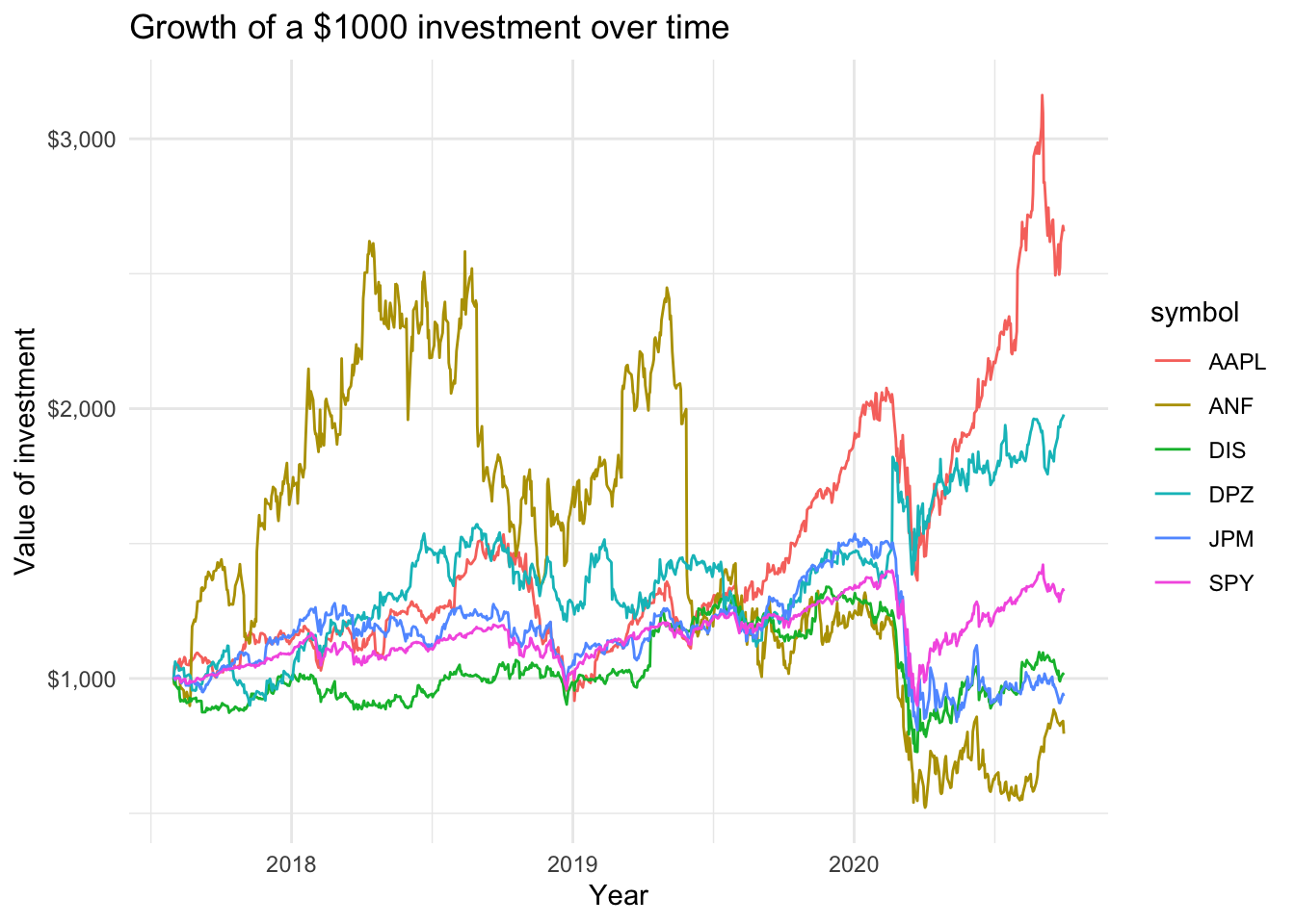
We may want to see what our investments would have grown to, of we had invested $1000 in each of the assets on Aug 1, 2017.
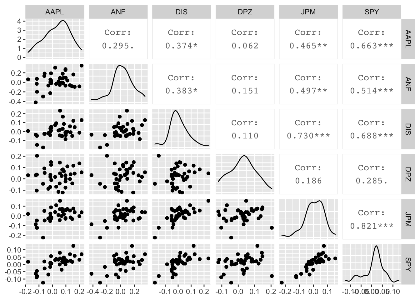
Scatterplots of individual stocks returns versus S&P500 Index returns.
Besides these exploratory graphs of returns and price evolution, we also need to create scatterplots among the returns of different stocks. ggpairs crates a scatterplot matrix that shows the distribution of returns for each stock, and a matrix of scatter plots and correlations. This may take a while to run, but look at the last row, the last column and along the diagonal.
The next step is to fit a liner regression model to calculate the \(\beta\) of AAPL. After fitting the model, we produce a summary table for the regression model, a 95% confidence interval for the coefficients, and an ANOVA table that shows the split of variability (Sum Sq) of AAPL returns and what portion ix explained by the market (SPY) versus the unexplained residuals.
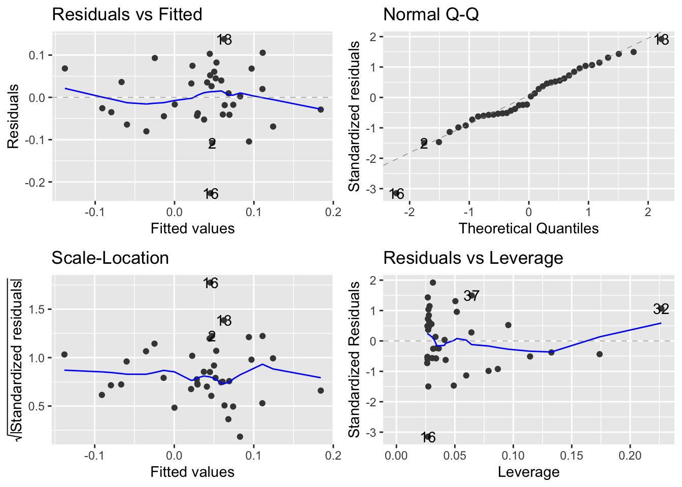
Besides fitting the model, we should also have a look at the residuals. Do they seem to follow a Normal Distribution? Is there a pattern in the residuals, or do they appear to be ‘random’? Is the variance of the residuals constant or does it seem to increase with increasing values of X?
First, we plot the residuals vs. the fitted (or predicted) values. This is a standard regression diagnostic plot to check whether there is no pattern in the residuals, as well as to test for heteroscedasticity, or whether the residuals appear to have unequal, non-constant variance.
The second thing we must check is whether the residuals follow a Normal distribution. A normal scores, or a QQ plot, allows us to check for skewness, kurtosis and outliers. (Note that the heteroscedasticity may show as apparent non-normality.)
ggplot(monthly_capm_returns, aes(x=SPY, y = AAPL))+
  geom_point()+
  geom_smooth(method="lm", se=FALSE)
## `geom_smooth()` using formula 'y ~ x'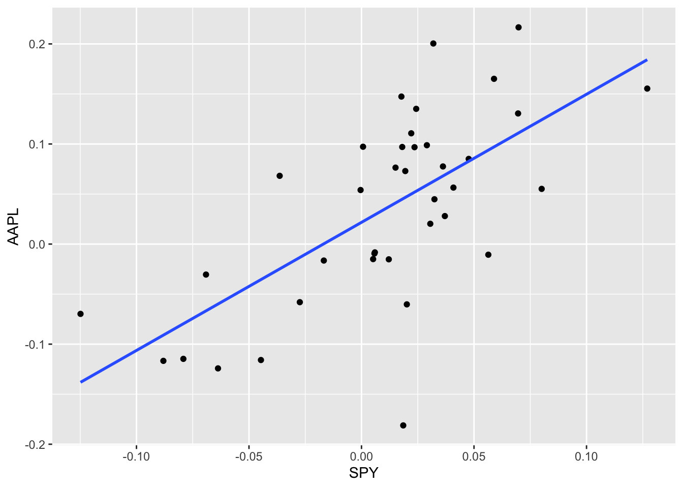
aapl_capm <- lm(AAPL ~ SPY, data = monthly_capm_returns)
mosaic::msummary(aapl_capm)
## Estimate Std. Error t value Pr(>|t|)
## (Intercept) 0.02170 0.01211 1.791 0.0816 .
## SPY 1.27993 0.24092 5.313 0.00000576 ***
##
## Residual standard error: 0.07296 on 36 degrees of freedom
## Multiple R-squared: 0.4395, Adjusted R-squared: 0.4239
## F-statistic: 28.22 on 1 and 36 DF, p-value: 0.000005763aapl_capm %>% broom::tidy(conf.int = TRUE)## # A tibble: 2 x 7
## term estimate std.error statistic p.value conf.low conf.high
## <chr> <dbl> <dbl> <dbl> <dbl> <dbl> <dbl>
## 1 (Intercept) 0.0217 0.0121 1.79 0.0816 -0.00287 0.0463
## 2 SPY 1.28 0.241 5.31 0.00000576 0.791 1.77aapl_capm %>% broom::glance()## # A tibble: 1 x 12
## r.squared adj.r.squared sigma statistic p.value df logLik AIC BIC
## <dbl> <dbl> <dbl> <dbl> <dbl> <dbl> <dbl> <dbl> <dbl>
## 1 0.439 0.424 0.0730 28.2 5.76e-6 1 46.6 -87.2 -82.3
## # … with 3 more variables: deviance <dbl>, df.residual <int>, nobs <int>autoplot(aapl_capm)